Sizing on-premises AI for your actual workloads
Size on-premises AI with representative requests, input lengths, peak concurrency, and service expectations instead of relying on employee counts.

Sarath Chandran

LLM inference sizing begins with the work the service must perform. Employee count alone cannot tell you which hardware, model, or serving configuration will meet that need. A hundred people submitting occasional short questions can create less demand than a scheduled document-processing job.
In enterprise IT capacity planning, procurement teams frequently make the mistake of sizing on-premises GPU clusters based solely on seat licensing metrics (e.g., "we have 5,000 corporate employees, so we need 5,000 user licenses and ten GPU servers"). In generative AI inference, user count is virtually meaningless without profiling request concurrency, prompt context token length, generation token length, and arrival distribution. A single automated document-processing batch job that ingests 50-page financial audits can consume more GPU memory bandwidth and compute FLOPS in ten minutes than an entire department of 500 knowledge workers asking brief interactive questions throughout an eight-hour shift.
Key Architecture Rule: Base GPU capacity sizing on two independent constraints: Memory Bandwidth Capacity (governing generation throughput and KV cache allocation) and Compute FLOPs (governing prompt prefill latency). Sizing for parameter weight storage alone guarantees Out-of-Memory (OOM) crashes under production concurrency.
Deconstruct the GPU VRAM memory equation
A common procurement disaster occurs when an organization purchases a 48GB GPU (such as an NVIDIA RTX 6000 Ada or L40S) to run a 70-billion-parameter quantized model, only to discover that the server crashes the moment three concurrent users submit prompts.
To size GPU hardware accurately, engineers must calculate total video memory (VRAM) allocation across four discrete consumers:
- Model Parameter Weights: The static memory required to hold model weights in memory. For a 70B parameter model:
- FP16 (16-bit): 70 × 2 GB = 140 GB (requires at least two 80GB H100s or four 48GB GPUs).
- FP8 (8-bit quantized): 70 × 1 GB = 70 GB.
- INT4 (4-bit quantized): 70 × 0.5 GB = 35 GB.
- Key-Value (KV) Cache Memory: The dynamic memory required to store past attention states for all active tokens across all concurrent user sessions. For multi-head attention models, KV cache scales linearly with context length and batch concurrency:
KV cache VRAM = 2 × layers × heads × head dimension × context length × batch size × bytes per elementIn a 70B model with a 16,000-token context window and FP16 precision, a single user session can require up to 4GB to 8GB of pure KV cache. Serving 10 concurrent users requires up to 80GB of VRAM dedicated purely to the KV cache, completely separate from the model weights! - Activation Memory & Workspace Buffers: Memory allocated dynamically for intermediate tensor calculations during matrix multiplication and attention scoring.
- CUDA Runtime Overhead: Baseline memory reserved by the NVIDIA CUDA driver and PyTorch execution context (typically 1GB to 2.5GB per GPU).
vLLM's optimization documentation details how PagedAttention partitions the KV cache into non-contiguous virtual memory blocks, eliminating external fragmentation and enabling significantly higher concurrency than naive transformers runtimes.
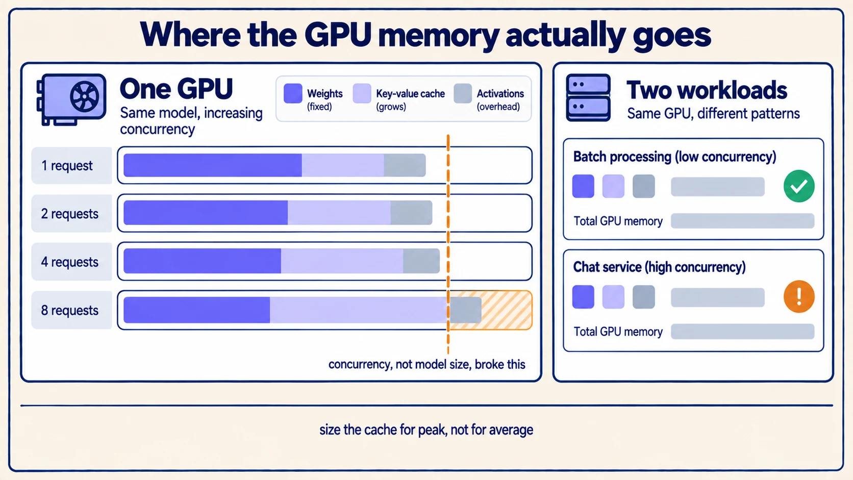
Two illustrative workloads with the identical user population
To illustrate why request characteristics dictate hardware architecture, examine two distinct enterprise workloads serving the exact same population of 200 corporate employees. The figures below are deliberately synthetic and illustrative; they do not represent measured benchmarks or vendor claims.
| Workload attribute | Scenario A: Interactive HR Policy Assistant | Scenario B: Automated Contract Extraction Queue |
|---|---|---|
| Active Employee Base | 200 registered enterprise users | 200 registered enterprise users |
| Typical Input Context | 1,200 tokens (policy FAQ + user question) | 16,000 tokens (multi-page commercial lease PDF) |
| Typical Generated Output | 200 tokens (concise conversational answer) | 1,200 tokens (detailed JSON schema extraction) |
| Request Arrival Distribution | Sporadic Poisson distribution throughout workday | Massive scheduled batch arrival at 6:00 PM daily |
| User Experience Target | Time to First Token (TTFT) < 800ms | Total batch completion window < 2 hours |
| Primary System Bottleneck | Prefill latency and streaming token responsiveness | KV cache capacity and sustained memory bandwidth |
| Recommended Serving Strategy | Low batch size, tensor parallelism for low latency | Continuous batching, high concurrency throughput |
In Scenario A, users require instantaneous conversational feedback. The hardware must prioritize low Time to First Token (TTFT) and high Inter-Token Latency (ITL) velocity. In Scenario B, no human is waiting on a screen; the priority is packing maximum concurrent requests into the GPU to maximize aggregate token throughput per dollar.
Attempting to run both workloads on an unpartitioned single-GPU server guarantees that when the 6:00 PM batch job fires, interactive users experience immediate 30-second conversational freezes.
Pro Tip: For interactive conversational agents, human readers perceive streaming output as "instantaneous" if the model achieves an Inter-Token Latency (ITL) of 30–50 milliseconds per token (equivalent to 20–33 tokens per second). Sizing hardware to achieve 150 tokens per second for a single conversational user yields diminishing human-perceived returns at massive hardware expense.
Establish service-level expectations before benchmarking
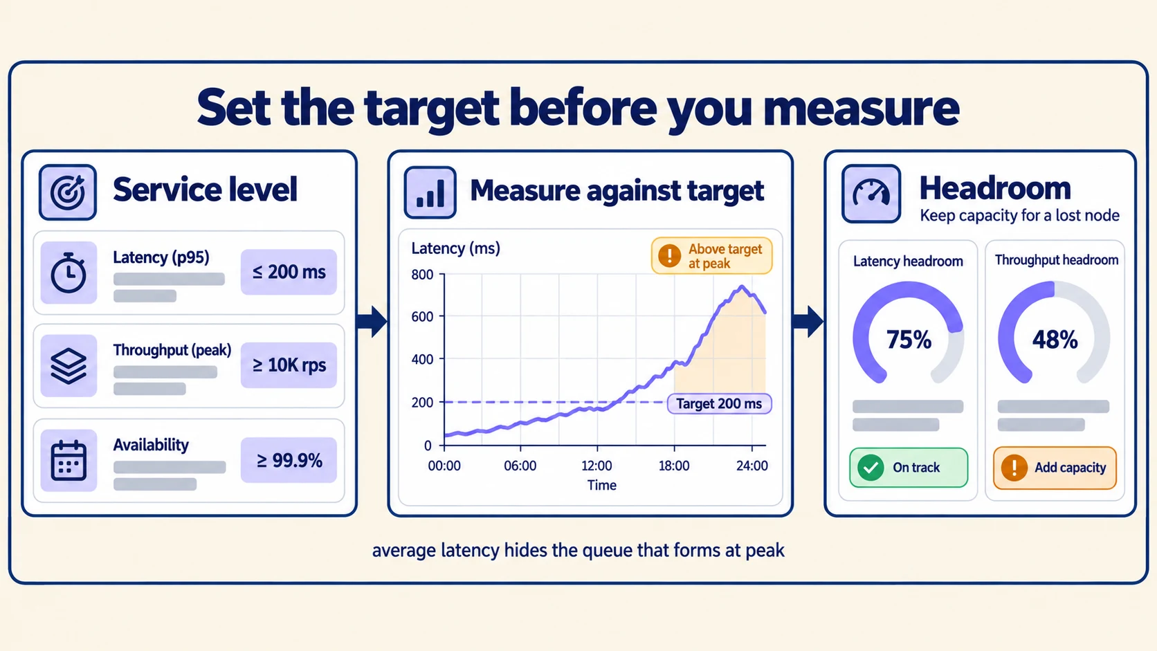
Prior to purchasing hardware or running load tests, platform engineering teams must establish quantifiable Service Level Objectives (SLOs) with business unit owners.
NVIDIA’s benchmarking metrics reference formalizes four core inference performance indicators:
- Time to First Token (TTFT): The latency from the moment a user submits a prompt to the moment the first generated token appears on screen. This measures the prefill phase (processing the input prompt).
- Inter-Token Latency (ITL): The time elapsed between consecutive generated tokens. This measures the autoregressive decode phase.
- End-to-End Request Latency (E2E): The total round-trip time required to complete the entire generation.
- Token Generation Throughput: The total aggregate tokens generated per second across all concurrent streams (tokens per second).
Establish clear P90 and P99 latency percentiles. A system that averages an acceptable 500ms TTFT but spikes to 14,000ms at the 95th percentile will suffer user rejection in production.
Build a reproducible, step-by-step benchmark plan
To size an on-premises cluster accurately, avoid theoretical math estimations; execute an empirical load test against candidate hardware using synthetic request distributions:
- Lock the Model & Serving Stack: Pin the exact model revision, precision quantization (FP16, FP8, or AWQ INT4), serving engine (e.g., vLLM or TensorRT-LLM), and host CUDA driver versions.
- Synthesize Representative Payloads: Create synthetic request datasets capturing short (500 tokens), median (2,500 tokens), and worst-case (16,000 tokens) prompt lengths.
- Measure Single-Stream Baseline: Run a single request to establish the minimum possible TTFT and ITL under zero contention.
- Step-Load Concurrency: Increase concurrent virtual users in controlled steps (1, 2, 4, 8, 16, 32, 64 concurrent streams) using realistic open-loop load generators (where requests arrive on independent Poisson intervals rather than waiting for previous responses).
- Plot the Saturation Knee: Identify the concurrency threshold where KV cache exhaustion forces the serving engine to queue requests, causing TTFT to degrade exponentially.
- Apply the 30% Operational Safety Margin: Establish the production capacity limit at 70% of the saturation point to absorb sudden workload spikes without triggering OOM crashes.
NVIDIA’s inference benchmarking analysis demonstrates why synthetic isolated benchmarks fail to predict real-world performance, emphasizing that multi-tenant production systems must be evaluated under mixed input-length concurrency.
Plan reserve capacity for high availability and failover
A hardware sizing plan that accounts only for steady-state peak load will fail during routine maintenance or hardware failures. If an enterprise requires four GPUs to serve peak daytime traffic, deploying exactly four GPUs leaves zero redundancy:
- N+1 Node Resilience: If a single GPU server crashes or requires an emergency driver update, can the remaining nodes absorb the traffic without violating SLOs?
- Quantization Tradeoffs: If scaling up physical GPU nodes is cost-prohibitive, consider deploying FP8 or INT4 quantization. Evaluating modern weight-only and activation quantization (such as AWQ or GPTQ) often recovers 40% to 50% of VRAM capacity with negligible degradation in reasoning benchmark accuracy.
- Failover & High Availability: Review our dedicated architecture guide on high availability for private AI to design resilient multi-node cluster topologies.
Furthermore, balance infrastructure sizing decisions against long-term operational expenditures, power consumption, cooling costs, and datacenter rack space using our comprehensive private AI total cost of ownership worksheet.
To explore model deployment requirements across leading architectures, consult our enterprise Model Hub and our foundational private AI deployment planning guide. When you are ready to evaluate sizing models against your organization's actual document workloads, schedule an enterprise architecture demo to review empirical hardware sizing models and benchmarking methodologies.